The Attractor Builder add-on was designed as a tool for numerical integration of differential equation systems and generating their trajectories directly inside Blender 4.5+. It allows users to run custom experiments, visualize attractors, export numerical data, and create fully animated 3D forms. The add-on is free and intended both for researchers working with dynamical systems and for artists who use attractors in graphics, animation, or generative art.

Installation
Recommended (Blender Extensions)
1. Open Blender and go to: Edit → Preferences → Extensions.
2. Search for Attractor Builder and click Install.
3. Enable the extension after installation.

Manual installation (from GitHub)
1. Download the attractor_builder.zip file from the GitHub repository.
2. In Blender, open: Edit → Preferences → Extensions.
3. Click Install from Disk… and select the downloaded .zip file.
4. Enable the extension after installation.

The add-on panel will appear in the N-panel → Attractor.

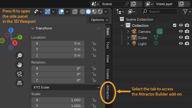
Interface
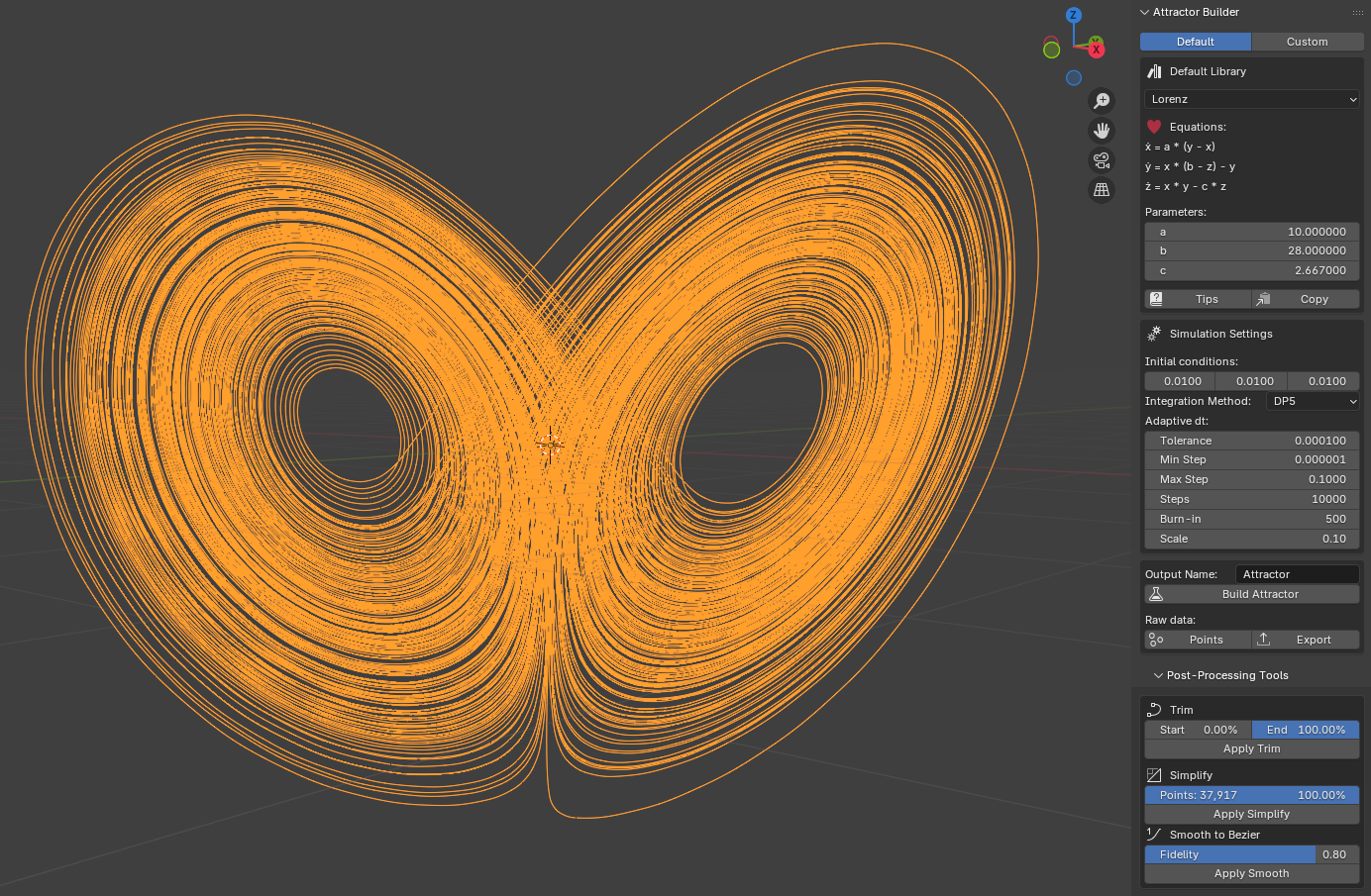
The Default tab provides access to the built-in library of systems (Lorenz, Chen, Lü, etc.) with predefined initial parameters. The Custom tab allows you to define your own equations and parameters.

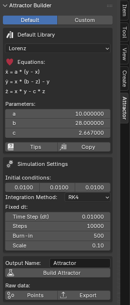
Default Library. A dropdown menu containing predefined attractor systems. After selecting a system, the corresponding equations and default parameters appear below. Equations: the system’s differential equations presented as three expressions representing the derivatives ẋ, ẏ, and ż. To ensure safety and consistency with the Custom mode, only the variables x, y, z are allowed, as well as the mathematical functions: sin, cos, tan, asin, acos, atan, sinh, cosh, tanh, exp, log, sqrt, pow, fabs. Standard arithmetic and unary operators are supported (+, -, *, /, **, %, and unary - and +). Parameters: a list of system parameters (e.g., a, b, c for the Lorenz system), which can be modified to influence the resulting trajectory. The Tips button provides short hints, and Copy transfers the equations and current parameters into the Custom mode for further editing.

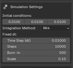
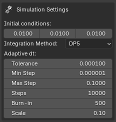
Simulation Settings. A group of simulation settings: initial state, integration method, and related parameters. Initial conditions: The starting coordinates x₀, y₀, z₀, from which numerical integration begins. Integration Method. A dropdown menu for selecting the numerical method (Euler, Heun, RK4, RKF45, DP5):

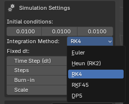
Fixed dt. For fixed-step methods (Euler, Heun, RK4), the available settings are: the time step Time Step (dt), the number of integration steps Steps, the warm-up phase Burn-in, and the scaling factor Scale.

Adaptive dt. Includes two adaptive methods (RKF45 and DP5) in which the user does not specify a fixed time step. Instead, the algorithm adjusts dt automatically based on the error tolerance Tolerance and the allowed range Min Step and Max Step.

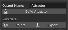
Output. The Build Attractor button generates a trajectory as a Curve object (specifically a Poly Curve) named according to the Output Name field — default: Attractor. Only after building the attractor does the Raw data section become available. The Points button creates a Mesh object named RawPoints, allowing preview of all generated points. The Export button saves the data to a CSV file for further analysis in Python, MATLAB, or Excel. The CSV file contains the columns steps, dt, x, y, z. Row 0 corresponds to the initial conditions provided in the Initial conditions section. Subsequent rows contain the points of the trajectory obtained at consecutive integration steps. The dt column is especially important for adaptive methods where the time step is computed dynamically.

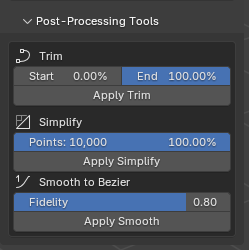
Post-Processing Tools. This section becomes available after the attractor is generated and allows simple post-processing of the resulting curve. The Trim tool shortens the trajectory by removing its beginning or end, using the Start and End sliders; clicking Apply Trim updates the curve permanently. The Simplify tool reduces the number of points of the Poly Curve, making the object lighter and easier to edit; this operation is independent of trimming. The Smooth to Bezier tool converts the polyline into a Bézier curve using a built-in smoothing algorithm, whose intensity is controlled by the Fidelity parameter. All three tools help prepare the trajectory for further editing, animation, or rendering.

Custom. This mode allows defining and saving custom systems of differential equations, which can then be integrated and visualized just like the systems from the built-in library. It is designed for users who want to experiment with their own models, modify existing systems, or document different parameter variants.

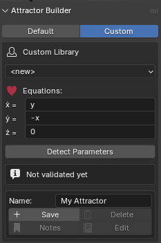
Custom Library. A dropdown list showing previously saved systems together with their parameters. Entries appear in reverse chronological order, making it easy to return to recently edited models. When entering your own equations, remember that the parser accepts only a safe subset of expressions: variables x, y, z; the mathematical functions sin, cos, tan, asin, acos, atan, sinh, cosh, tanh, exp, log, sqrt, pow, fabs; and the standard arithmetic operators +, -, *, /, **, %, as well as unary + and -. Any other syntax will be rejected.

Detect Parameters. This button analyses the entered equations, detects all symbols (excluding x, y, z), and generates the corresponding parameter list. This step is mandatory — without parameter detection and correct equation structure, the simulation cannot be started. After successful detection, parameters appear in the table below, where they can be assigned values just like in the Default mode.

Save/Notes/Edit/Delete. Once parameters are detected, the system can be saved under any name, adding it to the Custom Library. All saved systems are stored in a single .json file inside the add-on, so they remain available across Blender sessions. Users may attach notes to each saved system, such as origin descriptions, stability observations, typical parameter values, or numerical experiment results. The Note and Edit buttons allow viewing and editing notes, while Delete removes the system together with its notes from the JSON file.